Introduction
In my last post, I used Hansen’s Global Forest Change dataset to identify deforestation in Malawi. While global datasets may be convenient and comprehensive, they often overlook local circumstances. In this post, I identify tree cover in a study site in Cameroon by training my own random forest classifier. I then compare my results with Hansen’s, illustrating the value of training classifiers locally.
Analysis
I first created a class schema of 6 land cover classes: forest cover, bare ground, water, cropland, shrubs, and other. I selected these classes because they were each prevalent in the landscape and including them helped distinguish between trees and other features. I then selected about 45 training points in each class and fit a random forest classifier.
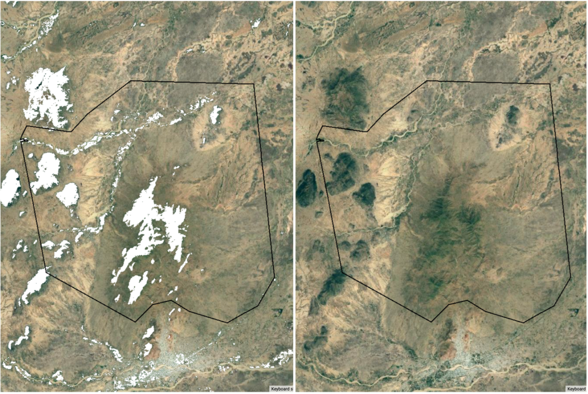
To determine the quality of my random forest classifier, I created two maps of my study area. The first map symbolizes the pixels which my random forest algorithm identifies as trees in white and outlines my study area in black. The second map displays Google’s base satellite imagery for the purposes of comparison with the ground truth.

Within my study site, my model performs relatively well, but far from perfectly. Feel free to Zoom in on specific clusters of trees using the Google Earth Engine link above. You will notice that some pixels are misclassified as trees and some pixels are failed to be classified as trees. These misclassifications are relatively common, especially along the rivers, along the edges of forested area, and in other sparsely forested areas. That said, where forests are dense my model performs very well, correctly classifying the bulk of each forested area. This pattern can be clearly seen in figure 1. Please note that my study area is but a fraction of the scene I worked with. Other regions in my scene perform far worse, with large swaths of water and fields misclassified as forests. Feel free to explore the rest of my scene at the link to my code above.
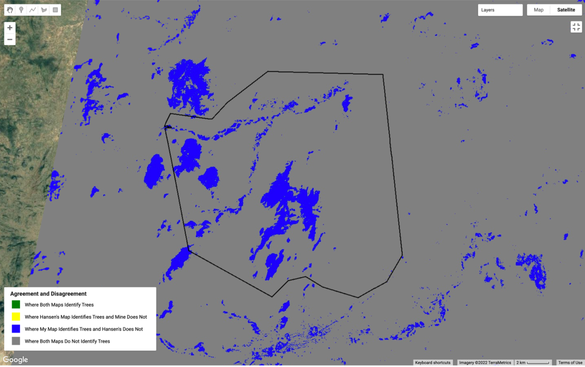
After classifying landcover in my study region, I imported Hansen’s Global Forest Change dataset to compare my tree cover classifier with Hansen’s. A map illustrating the agreement and disagreement between our two methodologies, where I define forests in Hansen’s dataset as pixels with greater than 30% tree cover, is illustrated in Figure 2.

Surprisingly, Hansen’s dataset does not identify any trees in the study region when I apply a standard definition of forest as at least 30% tree cover. Thus, figure 2 displays the pixels my classifier identifies as trees in blue and all other pixels in grey. This map makes it blatantly obvious that, at least at the 30% threshold, my classifier performs far better than Hansen’s. This makes sense to me. I trained my classifier specifically using the conditions present in my study area, while Hansen’s dataset attempts to apply one classifier to the entire world. Naturally, a local classifier should perform well where it was trained, as the global classifier does not account for the individuality of different regions.
Quantifying Performance of & Picking a Better Threshold for the Hansen Dataset
To quantify the performance of Hansen’s data in my study site, I used the following accuracy metrics using my classifier as the ground truth.
- True Positive Rate (TPR) = (# true positives)/(# true positives + # false negatives)
- True Negative Rate (TNR) = (# true negatives)/(# true negatives + # false positives)
- Balanced accuracy rate (BAR) = (TPR + TNR)/2
I calculated these metrics for eight different thresholds of percent tree cover, and my findings are summarized in the following table.
| Threshold | True Positive Rate | True Negative Rate | Balanced Accuracy Rate |
|---|---|---|---|
| 0% | 1 | 0 | 0.5 |
| 1% | 0.929 | 0.720 | 0.824 |
| 2% | 0.654 | 0.977 | 0.815 |
| 5% | 0.640 | 0.978 | 0.809 |
| 10% | 0.115 | ~1 | 0.558 |
| 20% | ~0 | ~1 | ~0.5 |
| 30% | 0 | 1 | 0.5 |
| 50% | 0 | 1 | 0.5 |
As the table shows, the highest TPR and BAR occur at a threshold of 1%. When the threshold is increased to just 2%, the TNR becomes very close to 1 but the TPR drops by almost 0.3, resulting in a slightly lower BAR. This pattern continues as the threshold is increased to higher percentages. I would experiment with thresholds between 1% and 2% in order to find a higher BAR, but unfortunately, this is not possible because Hansen’s treeCover band is reported as an integer. The best-performing percentage of tree cover in Hansen’s dataset is the 1% threshold.
Conclusion
Overall, these findings indicate that Hansen’s classifier performs so poorly in this part of Cameroon that the lowest possible indication of tree cover, 1%, performs the best. This just goes to show that massive world-scale models are not well-suited for localized studies. When working in a specific region, we tend to witness the highest performance when our models are trained in the region of our study.