Liam Smith's Portfolio
Research, remote sensing, GIS, and mathematics.
Spatial Accessibility of Healthcare Resources in Chicago
Introduction
In Rapidly Measuring Spatial Accessibility of COVID-19 Healthcare Resources: A Case Study of Illinois, USA, Kang et al. use the Enhanced Two-Step Floating Catchment Area (E2SFCA) method with parallel processing to assess the accessibility of ICU beds and ventilators to vulnerable populations – defined as individuals of 50 years of age or older – and COVID-19 patients in Illinois. The goal of their study was to provide policymakers with regularly updated information concerning the spatial capability of key treatment resources to COVID-19 patients and vulnerable populations. The authors found that access to ventilators and ICU beds was unevenly distributed throughout Illinois, and they published updated analyses daily in an online, interactive webpage called WhereCovid.
We seek to reproduce Kang et al.’s study for a few reasons. First, the global pandemic is a pressing issue, and public policy decisions regarding the pandemic ought to be based upon reputable research. Reproducing this study either confirms its findings, contributing to its validity as a basis for public policy, or overturns its findings, improving the basis of knowledge from which the government designs public policy. There are also intellectual and pedagogical motives for conducting a reproduction of this study. Intellectually, a reproduction confirms the validity of the researchers’ spatial techniques; and pedagogically, conducting a reproduction allows students to see how geospatial studies are conducted and encourages students think critically about their reputability.
Important Links
Materials and Methods
The Kang et al. study draws on four datasets:
- A hospital dataset provided by the Illinois Department of Health, which contains information about the number of ICU beds and ventilators at each hospital.
- A COVID-19 dataset also provided by the Illinois Department of Health, with information regarding the number of COVID-19 cases in each Zip Code in the state.
- A residential dataset from the 2018 American Community Survey 5 year table detailing the population and demographic composition of each tract in Illinois.
- A road network dataset queried from OpenStreetMap using the Python package, OSMnx.
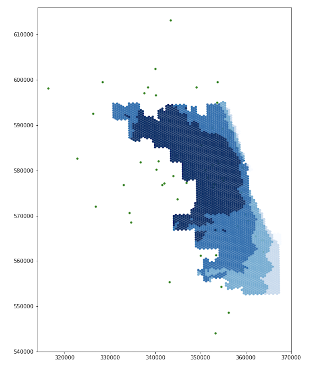
The provided research notebook includes only the data for the City of Chicago, because it is computationally burdensome for users to conduct this reproduction on the entire state of Illinois. In order to deal with boundary issues (i.e. sometimes the fastest route to a hospital in Chicago uses streets outside the city), a past GEOG 323 class revised the original methodology, extending the road network 15 miles past the boundaries of Chicago. However, the population data provided by the authors contained information exclusively for the tracts within Chicago. Residents of the Chicago suburbs can, and likely do, take advantage of the services provided by the hospitals physically within the city. For this reason, we know that a more accurate analysis would incorporate population information of Chicago’s suburbs.
In our class’s reproduction of this analysis, we seek to remedy this issue by extending the pool of demographic information to include the tracts in all of the counties neighboring Cook county, which is the county where Chicago is located. We did not address the geographic extent of the COVID-19 case data.
The computational resources available for the original study and our reproduction included a CyberGIS server and the programming language Python. Specifically, the study was conducted in a Jupyter notebook using the virtual computing environment, CyberGISX, a cyberinfrastructure project which performs computations on a bank of supercomputers at the University of Illinois Urbana-Champaign. Required Python packages include numpy, pandas, geopandas, networkx, OSMnx, shapely, matplotlib, tqdm, and multiprocessing.
Our Additions to the Code
To address our concern that individuals who live outside of Chicago might also use the hospital services within Chicago, we reconfigured the pre-processing of residential data in order to include households in the suburbs. Once we adjusted the input data, we simply re-ran the analysis to generate new results. Since the road network in the Jupyter notebook already included roads within a 15 mile buffer, we knew that the network analysis would work with our new residential dataset. Furthermore, since the code joins the centroids of census tracts that intersect catchment areas, we know that including superfluous residential information in our input dataset will not bring superfluous residential information into our results; residences that are located outside of the catchment areas simply are not counted. For this reason, we extended the pool of demographic information drastically, such that it includes the tracts in all of the counties neighboring Cook county.
Our additions to the code can be found in /procedure/code/04-Class-Reanalysis.ipynp under the “Population and COVID-19 Cases Data by County” subheading and our new figures are under /results/figures/reproduction and are copied below for convenience:
# Load data for tract geometry
tract_geom = gpd.read_file('./data/raw/public/ReanalysisClass/cb_2018_17_tract_500k.shp')
tract_geom.head()

# Load data for Census Demographics
tract_dem = pd.read_csv('./data/raw/public/ReanalysisClass/real_data_census_illinois.csv', sep=",", skiprows = [1, 1])
tract_dem.head()

# Extract the following columns: S0101_C01_001E, S0101_C01_012E, S0101_C01_013E, S0101_C01_014E, S0101_C01_015E, S0101_C01_016E, S0101_C01_017E, S0101_C01_018E, S0101_C01_019E
at_risk_csv = tract_dem[["GEO_ID", "NAME", "B01001_001E", "B01001_016E", "B01001_017E", "B01001_018E", "B01001_019E", "B01001_020E", "B01001_021E", "B01001_022E", "B01001_023E", "B01001_024E", "B01001_025E", "B01001_040E", "B01001_041E", "B01001_042E", "B01001_043E", "B01001_044E"]]
#Note: after a certain number of column names, atom becomes convinced that you're done with your code chunk. For this reason, I left out the last few columns in the code above, but they ought to be included when running the code.

# Find the number of columns in dataframe
len(at_risk_csv.columns)

# Sum all of the counts for individuals who are 50 years or older
at_risk_csv['OverFifty'] = at_risk_csv.iloc[:, 3:23].sum(axis = 1)

# create new pop column with a more useful name
at_risk_csv['TotalPop'] = at_risk_csv['B01001_001E']

# drop columns to clean the data set
at_risk_csv = at_risk_csv.drop(at_risk_csv.columns[2:23], axis =1)

# rename col to join
newnames = {"GEO_ID":"AFFGEOID"}
at_risk_csv = at_risk_csv.rename(columns = newnames)

# check projection
print(tract_geom.crs)

# transform CRS
tract_geom = tract_geom.to_crs(epsg=4326)

# check projection
print(tract_geom.crs)

# select tracts in Cook County and in counties adjacent to Cook County
tract_geom = tract_geom.loc[(tract_geom["COUNTYFP"] == '031')|
                            (tract_geom["COUNTYFP"] == '089')|
                            (tract_geom["COUNTYFP"] == '197')|
                            (tract_geom["COUNTYFP"] == '043')|
                            (tract_geom["COUNTYFP"] == '097')|
                            (tract_geom["COUNTYFP"] == '111')]

# perform an inner join based on AFFGEOID columns
atrisk_data = tract_geom.merge(at_risk_csv, how='inner', on='AFFGEOID')
Results and Discussion
Upon running the code with our updated residential dataset, we generated new figures, some of which differ significantly from the original results. Since we did not address the spatial extent of the COVID-19 case data, I am excluding COVID-19 accessibility maps from this report. The following maps reveal the accessibility of ICU beds and ventilators to vulnerable populations in Chicago. Darker blue represents higher spatial accessibility and lighter blue represents lower spatial accessibility.
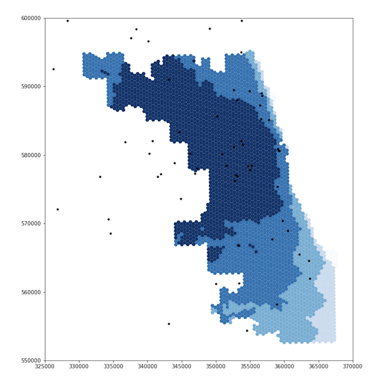
Accessibility of ICU Beds to Vulnerable Populations
Original Figure (after revisions by GEOG 323 Spring 2021)
Updated Figure
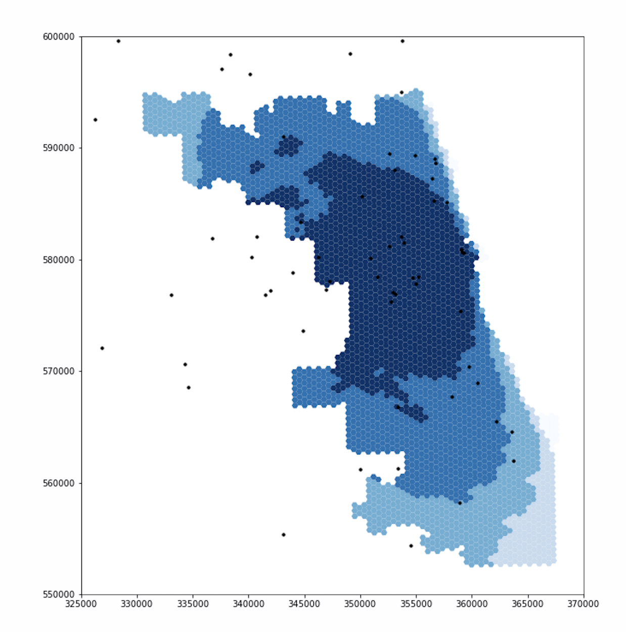 Note that the extents of the darker blues are much smaller in the updated figure, especially in the northwest and southwest.
The new figure also includes a section of light blue in the northwest, which was a darker shade in the original figure.
We will discuss these results further after reviewing the second set of figures.
Note that the extents of the darker blues are much smaller in the updated figure, especially in the northwest and southwest.
The new figure also includes a section of light blue in the northwest, which was a darker shade in the original figure.
We will discuss these results further after reviewing the second set of figures.
Accessibility of Ventilators to Vulnerable Populations
Original Figure (after revisions by GEOG 323 Spring 2021)
Updated Figure
 Similar to the first set of figures, the extents of the darker blues are smaller in the updated figure than in the original figure, especially in the northwest and southwest.
The new figure also includes a section of light blue in the northwest, where the original figure had been darker.
Similar to the first set of figures, the extents of the darker blues are smaller in the updated figure than in the original figure, especially in the northwest and southwest.
The new figure also includes a section of light blue in the northwest, where the original figure had been darker.
For both ICU beds and ventilators, the original and updated figures are similar on the east side, but differ significantly in the northwest and southwest. These differences makes sense. Because Chicago borders Lake Michigan on the east and it takes time to drive to hospitals, including adjacent counties in the residential dataset will not increase the population accessing hospitals in Chicago’s east side. With a similar number of people accessing hospital services, the spatial accessibility of those services remains similar for individuals who live in eastern Chicago. However, our adjusted residential dataset does impact the accessibility of hospitals for residents in western, northern, and southern Chicago. The hospitals in these parts of Chicago are less isolated from suburban residents, as they can drive to these hospitals in less time. Incorporating those suburban residents into our analysis increases the perceived demand for hospital services in western, northern, and southern Chicago. With more people accessing hospital services, it is more difficult for any one individual to access those services, and the spatial accessibility measure mapped by our figures declines accordingly.
The differences between the original and updated figures highlight the inaccuracies that boundary effects introduce to Kang et al’s results. In their paper, Kang et al include hospitals within 15 miles of the city, but not the residents. Since residents outside of the city also use hospitals within the city, the authors appear to have neglected an important boundary effect. Our updated analysis accounts for this issue and illustrates that the surrounding populations significantly impact the spatial accessibility of healthcare resources within the city.
If you would like more information regarding the processes and results of this reproduction, please see my complete reproduction repository here.
Conclusions
At the end of the day, we were able to reproduce the study and make minor improvements to the code. This would not have been possible for a group of undergraduate students to accomplish in a couple of afternoons had we not been provided the Jupyter notebook on CyberGISX. The Jupyter notebook illustrates exactly how the authors addressed their research questions and provides some information as to the motivations for their choices, making it possible to review their code and methodology in a manner that is impossible for most research papers. Cudos to the authors for their foresight in publishing their work in a cutting-edge, reproducible environment.
Conducting the reproduction, however, also introduced me to the limitations and errors in their work. Discovering that their analysis of Chicago included hospitals but neglected the road networks and population outside of the city was surprising and somewhat eye-opening. The authors of the study are some of our top geospatial researchers, and they still made mistakes. If anything, this reproduction drew my attention to the importance of reproducing academic studies. All of us, even those at the top of the field, make mistakes, and a thorough peer review process is critical to addressing those errors.
Another key takeaway is that undocumented pre-processing of data poses significant barriers to reproducibility. While the authors performed some manipulations on their data simply to format it for the study, they do not document those manipulations in their code. For this reason, when we extended the geographic extent of the residential database, we had no model to work off of and had to develop our own method.
Overall, Kang et al’s study on spatial accessibility of COVID-19 healthcare resources is reproducible, and their Jupyter notebook on CyberGISX provides the public with all of the information necessary to computationally reproduce their analysis in Chicago. There are, however, a couple areas in which the work could be improved. Future work on the notebook could include documenting their data preprocessing and adding more comments to their code to make it easier to assess their methodology. Additionally, to account for the fact that residents outside of Chicago (which we added in this revision) could also access the hospitals outside of the city that are included in this analysis, the road network ought to be extended even further. Since hospital catchment areas are 30 minutes of driving time, extending the road network 60 miles past the boundary of Chicago would be adequate. Further than that distance, even an individual traveling at the maximum speed limit in a straight line would not be included in any catchment areas, so they would be irrelevant to our analysis. This Jupyter notebook is already an incredibly valuable tool for teaching and learning the methods of reproducible GIS, and continual work on the notebook will only continue to improve its functionality.